How Real Options Flexibility Boosts NPV: Theory + Example

Real options increase the expected returns of an investment opportunity by allowing adjustments to the investment strategy in response to changing market conditions or new information.

In other words, having more flexibility in investment and disinvestment increases the value of a project. Why? Because by considering exit options at the start of a project, managers can better evaluate risk and uncertainty, which ultimately leads to higher returns.

In this post, we’ll look at 8 increasing levels of flexibility and how they improve the NPV of a project.

Ready? Let’s dive right in:

What are Real Options

When evaluating a new project, it’s important to consider the option to close the project in the future, as this can add significant value to the project.

Failing to do so leads to missing out on what could be good investment opportunities.

The most commonly used decision rule for investment projects is the Net Present Value (NPV), which compares the risk-adjusted present value (PV) of expected cash inflows to that of outflows.

While the NPV method overcomes flaws of other rules, it assumes managers will do nothing if circumstances change, which is rarely the case in the real world.

The conventional NPV treats the investment decision as a static commitment that you can’t change.

In reality? As market conditions worsen, businesses respond by either altering or even shutting down projects.

But how can you value this liberty?

Real options theory uses the Black-Scholes-Merton financial option pricing model to value the future managerial flexibility of real-world projects.

You see, the more flexibility managers have to change their past decisions, the higher the value of the project.

See also: Examples of Real Options (3 Full Numerical Case Studies)

#1) Static NPV

Static NPV (also called conventional NPV) is the commonly used basic method for evaluating investments based on fixed assumptions about the future.

This method assumes the decision to invest is irreversible. The company can either invest today, or never do so again.

Again, it doesn’t account for the option managers have to change the production level or abandon a project if market conditions change or if new information becomes available.

To put these concepts in motion, we’ll follow the same example across a series of levels of flexibility. Imagine a company has a project with the following characteristics:

• Initial investment cost: $15M
• Present value of expected future cash flows: $16M

The static NPV is straightforward—subtract the investment cost from the PV of cash flows. -15+16=$1M.

Additionally, the time to expiration is 10 years—you can think of it as the window of opportunity to make the project happen. The uncertainty (volatility, or σ) of the project’s value and its cash flows is 20%. The risk-free interest rate is 6%. And the dividend yield (rate of return shortfall) is 5%.

Now, you may be wondering what some of these things mean:

Key Concepts

Before we start measuring the value of flexibility, it’s important to go through some important definitions first:

• Operating state: When the firm decides to invest in the project and start generating cash flows. In this state, the firm pays the costs associated with running the project, but also receives revenues from its operations.
• Idle state: When the firm decides not to invest in the project. In this state, the firm incurs no investment costs but also generates no cash flows.
• V: Value of the project. It evolves over time through a Geometric Brownian Motion (more on this below).
• Boundary: The value of the project at which the firm should invest (call option) or divest (put option). You calculate it by solving for the optimal exercise point of an option to invest or disinvest in the project, where the option value is equal to the net present value of waiting to exercise. The boundary can be an output price, investment cost, or volatility, for example.
• Time to expiration: The remaining time until an option contract expires. This is an important factor in the value of an option, as it affects the likelihood of the investor exercising it. The longer the time to expiration, the greater the potential benefits of exercising the option, but also the greater the potential costs associated with delaying the decision.
• Rate of return shortfall: Also called the convenience yield (and the equivalent to a stock’s dividend yield). It refers to the difference between the rate of return on an underlying asset and the rate of return you get from holding an option on that asset. In other words, it’s the benefit the owner of the underlying asset collects, but not the owner of the option. A positive rate of return shortfall is important because it implies a non-zero cost of waiting for investment opportunities—while waiting for an investment opportunity to become available, the firm doesn’t receive the benefits associated with owning and operating the project (underlying asset). If there is no dividend (no cost of waiting to invest), you can delay the project forever because it’s never optimal to exercise early (the American-style option becomes equal to its European equivalent). The problem with this? It is unrealistic.

You can value options using a continuous-time model, or a discrete-time model.

The difference?

A model that uses continuous time measures the timing of decisions and the cash flows of a project continuously over time, as opposed to discretely at specific time intervals (such as the binomial option pricing model).

In continuous time models such as the Black-Scholes-Merton (BSM) model, the value of an investment changes smoothly. This gives you a more accurate representation of the complex and unpredictable nature of investment projects.

The BSM follows a Geometric Brownian Motion (GBM), a mathematical model that simulates a large number of possible future scenarios for the project value, and estimates the probability of different outcomes along with the costs and benefits of each.

We’ll use the BSM model throughout the example.

#2) Forward Start NPV

As the name implies, this is similar to a forward contract rather than a financial option.

The company is forced to invest in a project at a predetermined future date. Hence, it has limited flexibility (if we can call it flexibility at all).

Still, it is superior to the static NPV because allows the firm to delay the start of the investment project until a future date.

To compute it, you first assume the initial investment cost is not paid today, but at the predetermined future date. And also that the PV of expected future cash flows was discounted to that date.

Then, you discount the initial investment costs to the present, as well as the expected future cash flows:

\[V_te^{-q\tau}-Xe^{-r\tau}=16000\cdot e^{-0.05\cdot10}-15000\cdot e^{-0.06\cdot10}=1472.32\]

Where:

• V_t is the present value of the expected cash flows of the project.
• q is the rate of return shortfall.
• τ (greek letter Tau) is the time to expiration. In other words, the remaining time until the option contract expires (T being the expiration date).
• X is the investment cost for the project.
• r is the risk-free interest rate.

Despite its limited flexibility, the forward start NPV is $1.5M, significantly larger than the static NPV of $1M (and this is just the first level of flexibility).

The cash flows are discounted at the dividend yield, while the investment cost is discounted at the risk-free rate. Why?

Remember, the PV of the project’s cash flows is the equivalent of the underlying asset price in a financial option. While the strike price is the investment cost.

By delaying the investment cost, it means you have that money available until you decide to invest—so you can deposit it earning the risk-free interest rate in the meantime.

As to the PV of cash flows, the positive rate of return shortfall means the project value increases over time. This means you need to buy fewer “units of the underlying asset” today to have the desired amount by the time you decide to invest (put-call parity with continuous dividends).

#3) European Call Option NPV

Now let’s imagine that upon the expiration date, the firm has the option to invest or not.

This is an European-style call option, right?

Unlike the forward, an option gives the company the right (but not the obligation) to invest.

To compute this, you need to be familiar with the Black-Scholes model.

You start by making the cumulative normal distribution computations:

\[d_1=\frac{ln(\frac{V_t}{X})+(r-q+\frac{\sigma^2}{2})T}{\sigma\sqrt{T}}=\frac{ln(\frac{16000}{15000})+(0.06-0.05+\frac{0.20^2}{2})10}{0.20\sqrt{10}}=0.5764\] \[d_2=d_1-\sigma\sqrt{T}=0.5764-0.20\sqrt{10}=-0.0561\]

Next, you want the probability of the underlying asset price being above the strike price of the option at the expiration date.

To do that you can take the values of the d₁ and d₂ parameters to a standard cumulative normal distribution table, you can use the Excel function NORMSDIST, or you can use a calculator.

You’ll find that N(d₁) is 0.7190 and N(d₂) is 0.4761.

Plug everything into the magical BSM formula to get the European call option price:

\[c_t=V_t\cdot e^{-qT}\cdot N(d_1)-X\cdot e^{-rT}\cdot N(d_2)=16000\cdot e^{-0.05\cdot10}\cdot0.7190-15000\cdot e^{-0.06\cdot10}\cdot0.4761=3058.19\]

Thus, the value of the project considering an option to invest either today or at the expiration date is $3.1M—significantly greater than both the forward start NPV and the static NPV.

#4) American Call Option NPV

Here we increase the flexibility up a notch. The firm now has the option to invest at any time between today and the expiration of the option.

An European call option gives you less flexibility than an American call option because you can only exercise it at a fixed point in time—the expiration.

But this difference is only relevant when the rate of return shortfall is positive.

If you remember from financial options, the price of an American call on a stock that doesn’t pay dividends is equal to the price of its European-style option equivalent. Why?

Because zero dividend means it will never be optimal to exercise the option early, as you’re not missing out on anything for having the option as opposed to the asset.

Now, this makes the option pricing problem more complex. The problem?

You can’t use an easy closed-form solution like the Black-Scholes model to accurately solve this option pricing model.

You’d either have to use more intensive methods such as the binomial option pricing model (with thousands of time steps) or a Monte Carlo simulation in a program such as MATLAB, which is beyond the scope of this post.

The example we’re following throughout the post is adapted from a set of lecture notes. Following those notes, we’ll consider the American-style call option NPV as $3.6M.

#5) Perpetual Irreversible NPV

From here on, we’ll look at projects with an infinite stream of cash flows for which we’ll want the present value.

The perpetual irreversible NPV is the net present value of a project you can exercise indefinitely—but can’t reverse or abandon once you have undertaken it.

This type of investment opportunity is characteristic of assets such as real estate, natural resources, or infrastructure projects—that have long useful lives and generate cash flows over an extended period of time.

We are dealing with a perpetual option to invest. In other words, the option’s time to maturity is infinite—as opposed to the 10 years we saw before.

To find the project value, you compute the price for a perpetual American-style call option.

Now, an infinitely-lived continuously-exercisable American-style option is unrealistic.

It would only happen in reality with a monopolistic company whose competitors would never be capable of doing a similar project.

Still, studying an infinite option helps you understand more complex concepts later.

The goal now is to understand when is the optimal time to invest—since you can do so at any time.

In other words, at what time is it optimal to invest a sunk cost X̅ whose return is a project with a value of V?

Thus, the firm needs to decide whether to continue in the idle state or to enter the market by exercising this American option to invest.

For this investment decision problem, you start by identifying a barrier V̅—that represents the project value at which it is optimal to invest.

Remember, the investment cost is fixed, but the PV of its cash flows (project value) evolves through a GBM.

V̅ is the boundary that separates the continuation region (stay in the idle state) from the exercise region (move to the operating state). By investing in the project the firm receives a net payoff worth V̅ – X̅. This is called the value-matching condition.

Now, how do you determine V̅?

Consider the value function F(V):

\[F(V)=\begin{cases}(\overline{V}-\overline{X})(\frac{V}{\overline{V}})^{\beta_1} & V

Where the entry threshold V̅ is given by:

\[\overline{V}=\frac{\beta_1}{\beta_1-1}\overline{X}\]

And β₁ (the elasticity parameter) is:

\[\beta_1=\frac{1}{2}-\frac{r-q}{\sigma^2}+\sqrt{(\frac{r-q}{\sigma^2}-\frac{1}{2})^2+\frac{2r}{\sigma^2}}>1\]

Wondering where do these formulas come from?

To accurately reflect the characteristics of this investment opportunity, the solution to this perpetual American option pricing problem considers the following boundary conditions:

• If the value of the project touches zero, it will stay there forever and the option has no value. In other words, if the present value of cash flows is very small, the firm has no reason to exercise its option to invest and enter the market.
• Value-matching condition, mentioned above.
• Smooth-pasting condition (also called high-contact condition): It is a mathematical constraint that ensures the continuity and differentiability of the F(V) value function and its first derivative at the point where it is optimal to exercise the option. The goal? To ensure there are no discontinuities in the value of the investment.

Now, the elasticity parameter β₁ should always be higher than 1. Why?

Because it is one of the two roots of the quadratic equation. We will define the other root later as β₂, which must be always lower than 0.

This guarantees a convergence condition that translates into a positive cost of waiting (rate of return shortfall), but explaining it in detail is beyond the scope of this post.

Let’s see the investment strategy visually:

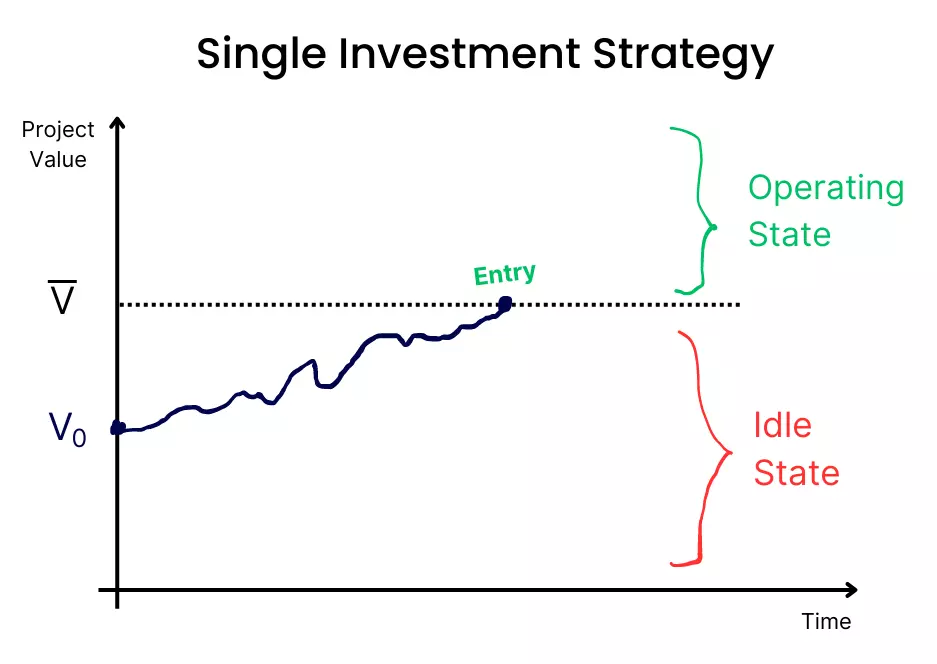
As pictured above, when V < V̅, it is not yet optimal to exercise the option to invest.

Finally, let’s plug the numbers from our example into these formulas to get the NPV considering this new level of flexibility.

Starting with the elasticity parameter:

\[\beta_1=\frac{1}{2}-\frac{0.06-0.05}{\sigma^2}+\sqrt{(\frac{0.06-0.05}{\sigma^2}-\frac{1}{2})^2+\frac{2\cdot 0.06}{\sigma^2}}=2\]

And now the investment threshold V̅:

\[\overline{V}=\frac{2}{2-1}\cdot 15000=30000\]

V̅ ($30M) is above V ($16M, the PV of cash flows), which means the firm is in the continuation region and it’s not yet optimal to exercise the option.

Thus, you use the upper part of the F(V) equation to get the perpetual irreversible NPV of around $4.3M:

\[(30000-15000)(\frac{16000}{30000})^{2}=4266.67\]

Starting to notice the pattern? As managerial flexibility increases, so does the NPV.

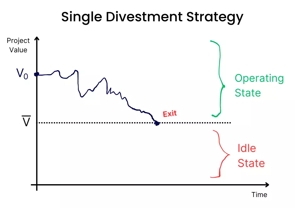
We can also apply this to divestment decisions:

Perpetual American-Style Put Option Pricing Solution

This is when the firm is already in the project after paying the initial investment, but has the option to discontinue it at any time.

Here, V̅ and X̅ (investment costs of the project) are replaced by V̲ and X̲:

• V̲: Optimal decision to divest.
• X̲: Value the company receives in the future if it abandons operations, which is assumed to be known and fixed. It represents the divestment proceeds the firm can recoup by exercising the shutdown (or abandonment) option.

And the solution to F(V) becomes:

\[F(V)=\begin{cases}(\underline{X}-\underline{V})(\frac{V}{\underline{V}})^{\beta_2}&V>\underline{V} \\ \underline{X}-V & V\leq\underline{V}\end{cases} \\ \underline{V}=\frac{\beta_2}{\beta_2-1}\underline{X}\\\beta_2=\frac{1}{2}-\frac{r-q}{\sigma^2}-\sqrt{(\frac{r-q}{\sigma^2}-\frac{1}{2})^2+\frac{2r}{\sigma^2}}

Here, we consider that if the project value goes to infinity, the option to abandon is worthless. In other words, if the present value of cash flows is very high, the firm has no reason to stop the project. Makes sense, right?

Also, under the value-matching condition, by divesting, the firm receives X̲ – V̲. The smooth-pasting condition applies as well.

#6) Perpetual NPV with an Option to Exit

Under the perpetual irreversible NPV, the firm stays in the operating state forever once it makes the investment. There’s no option to abandon.

But in reality? Firms can shut down operations if market conditions become unfavorable.

Therefore, it’s also important to analyze how much the flexibility to exit a project increases the NPV.

So, consider the firm has an investment opportunity with an option to exit after.

In other words, this is an option to invest with a subsequent option to divest later and recover a given amount—and it results in two optimal trigger points:

• V̅: Optimal decision to invest.
• V̲: Optimal decision to divest.

Continuing the example, let’s say X̲—the amount the firm recovers after exiting the project—is $14M.

Now you can calculate α, the recovery rate. When this value is one (100%), the firm recovers everything it invested. If it’s zero, the firm recovers nothing.

In our example, the firm recovers 15/14=93% of the initial investment.

The compound option of investment with a subsequent option to exit is equal to:

\[F(V)=\begin{cases}(\overline{V}+(\underline{X}-\underline{V})(\frac{\overline{V}}{\underline{V}})^{\beta_2}-\overline{X})(\frac{V}{\overline{V}})^{\beta_1} & V

Where the investment threshold V̅ is the solution to the equation:

\[(\beta_1-\beta_2)(\underline{X}-\underline{V})(\frac{\overline{V}}{\underline{V}})^{\beta_2}+(\beta_1-1)\overline{V}-\beta_1\overline{X}=0\]

Continuing the example, start by computing β₂ using the formula we saw in the American put option:

\[\beta_2=\frac{1}{2}-\frac{0.06-0.05}{0.20^2}-\sqrt{(\frac{0.06-0.05}{0.20^2}-\frac{1}{2})^2+\frac{2\cdot 0.06}{0.20^2}}=-1.5\]

From there, you can compute the divestment threshold V̲:

\[\underline{V}=\frac{-1.5}{-1.5-1}14000=8400\]

As to the investment threshold V̅ for this compound option to invest (call) with an option to exit (put) after, you need to solve the following equation using your calculator, Excel’s Solver, or by hand if you’re courageous enough:

\[(2-(-1.5))(14000-8400)(\frac{\overline{V}}{8400})^{-1.5}+(2-1)\overline{V}-2\cdot 15000=0 \\ \Leftrightarrow \overline{V}=26503\]

Since V̅ ($26.5M) is bigger than V ($16M), you use the first branch of the F(V) equation:

\[F(V)=(26503+(14000-8400)(\frac{26503}{8400})^{-1.5}-15000)(\frac{16000}{26503})^{2}=4557\]

Thus, the Perpetual NPV with an option to exit is worth $4.6M.

#7) Perpetual Costly Reversible NPV

Costly reversible NPV refers to a type of investment project where there is a cost to undoing the project.

In other words, if the manager decides to abandon the project at some point in the future, it would require a significant investment of resources to do so.

If V exceeds the upper threshold V̅, it is optimal for the firm to switch from idle to the operating state. Conversely, if V falls below the lower threshold V̲, it is optimal for the firm to switch from the operating to the idle state.

These two time-independent values create a range where nothing happens (often called the hysteresis band) and that determines when it is optimal to switch between the idle and the operating state.

How does this work practically?

When the value of the project rises above the optimal intervention level V̅, the (monopolistic) firm exercises the (call) option to start the project. To do so, it also pays the switching or investment cost X̅.

What does the firm get in exchange?

An operating project and a (put) option to exit that project if market conditions worsen in the future. V̲ is the level at which the firm exercises that put option. In return? It receives the disinvestment proceeds X̲ and a (call) option to re-enter again.

And the cycle continues forever, unlike the perpetual NPV with one option to exit.

Now, how do you calculate the trigger values V̅ and V̲? You need a couple of items we computed previously:

• α (93%), the recovery rate you saw previously, which can now be interpreted as the ratio of switching costs.
• β₁ elasticity parameter, which must always be greater than 1. In this case, we saw it is 2.
• β₂ elasticity parameter, which should always be negative. In this case, we calculated it previously and it was -1.5.

With these, you can calculate γ (Gamma)—which you can interpret as the ratio of the lower to the upper optimal intervention thresholds—by solving the following equation:

\[\alpha=\frac{\beta_1\beta_2(\gamma^{\beta_2+1}-\gamma^{\beta_1+1})+\beta_2\gamma^{\beta_1+1}-\beta_1\gamma^{\beta_2+1}+(\beta_1-\beta_2)\gamma^{\beta_1+\beta_2}}{\beta_1\beta_2(\gamma^{\beta_2}+\gamma^{\beta_1})-\beta_2\gamma^{\beta_2}+\beta_1\gamma^{\beta_1}-(\beta_1-\beta_2)\gamma} \\ 0.93=\frac{2(-1.5)(\gamma^{(-1.5)+1}-\gamma^{2+1})+(-1.5)\gamma^{2+1}-2\gamma^{(-1.5)+1}+(2-(-1.5))\gamma^{2+(-1.5)}}{2(-1.5)(\gamma^{(-1.5)}+\gamma^{2})-(-1.5)\gamma^{(-1.5)}+2\gamma^{2}-(2-(-1.5))\gamma} \\ \Leftrightarrow \gamma=0.5071\]

So, for every recovery rate, the ratio of the lower to the upper trigger is retrieved from the equation above.

Next, you can calculate the optimal thresholds V̅ and V̲:

\[\overline{V}=\beta_1\beta_2(\gamma^{\beta2}-\gamma^{\beta1})\frac{\overline{X}}{\beta_1\beta_2(\gamma^{\beta2}-\gamma^{\beta1})-\beta_2\gamma^{\beta_2}+\beta_1\gamma^{\beta_1}-(\beta_1-\beta_2)\gamma}=24347 \\ \underline{V}=\beta_1\beta_2(\gamma^{\beta2}-\gamma^{\beta1})\frac{\underline{X}}{\beta_1\beta_2(\gamma^{\beta2}-\gamma^{\beta1})+\beta_2\gamma^{\beta_1}-\beta_1\gamma^{\beta_2}+(\beta_1-\beta_2)\gamma^{\beta_1+\beta_2-1}}=12347\]

Along with the option constant C1:

\[C_1=\frac{\overline{V}}{\beta_1\beta_2(\gamma^{\beta_2}-\gamma^{\beta_1})}\beta_2(\gamma^{\beta_2}-\gamma)\overline{V}^{-\beta_1}=0.00001849\]

Finally, to get the perpetual costly reversible NPV of $4.7M, you simply:

\[NPV=C_1V^{\beta_1}=0.00001849\cdot16000^2=4734\]

#8) Perpetual Costless Reversible NPV

In the previous section, reversing the investment is pricey. In other words, the firm recovers only a portion of the initial cost, hence α (recovery rate) is between 0 and 1.

In the previous previous section, the irreversible NPV states the company recovers zero percent of the investment, meaning X̲ = 0 and thus, α = 0.

Now?

We’ll look at the perfectly reversible case, where α = 1. This means the money recovered with the disinvestment is equal to the cost of setting up the project (X̲ = X̅ = X̲̅ = $15M).

Furthermore, the hysteresis band disappears because there’s a single threshold for both the activation and deactivation of the project.

In other words, the level of project value at which investment and disinvestment occur are no longer separated. The result?

V̅ and V̲ are now determined simultaneously, as opposed to exponentially like in the previous levels of flexibility:

\[\overline{\underline{V}}=\frac{\beta_1\beta_2}{\beta_1\beta_2-(\beta_1+\beta_2)+1}=\frac{r\overline{\underline{X}}}{q}=\frac{0.06\cdot15000}{0.05}=18000\]

The perpetual costless reversible NPV is equal to:

\[NPV=\begin{cases}\overline{\underline{V}}\frac{\beta_2-1}{\beta_1(\beta_2-\beta_1)}(\frac{V}{\overline{\underline{V}}})^{\beta_1} & V\overline{\underline{V}}\end{cases}\]

Since V ($16M) is lower than V̲̅ ($18M), you use the first branch of the equation above to get an NPV of $5.1M:

\[NPV=18000\frac{-1.5-1}{2(-1.5-2)}(\frac{16000}{18000})^{2}=5079\]

This is probably the largest NPV you could feasibly extract from the parameters in this example.

It represents the net present value of the investment opportunity assuming you can suspend and resume at no cost, and that you can do so an infinite number of times.

Notice how this combined entry and exit model is much larger than the classic NPV.

Key Takeaways

The main conclusion as you go through the various levels of flexibility is that the value of an investment opportunity increases with the level of flexibility.

Having more options to adjust the investment strategy allows managers to position their companies to capture the value of a new opportunity, or to cut short what turned out to be a bad one.

This greater flexibility allows for better risk management and can lead to higher returns.

Questions? Doubts? Feedback? Leave them in the comments below.