This is a basic introduction to understanding the logic behind the one-step binomial model. We won’t be going deep on the algebra.
This overview of the binomial option pricing model will help you understand the:
- Binomial trees widely used to price options and other derivatives.
- No-arbitrage argument used to value options.
- Reasoning behind different alternatives for replicating portfolios.
Let’s dive in:
What is a Binomial Tree?
A binomial tree is a diagram that illustrates different paths the stock price can follow over the life of an option.
Constructing a binomial tree is a useful way to price an option. It is a procedure widely used to value other derivatives as well.
In each time step, there’s a certain probability the stock will go up by a certain percentage, and a certain probability it will move down a certain % amount.
One-Step Binomial Model Example
Let’s look at an example of how to price a call option.
Consider a simple situation:
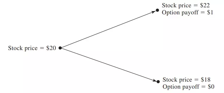
A stock trades at $20 today. 3 months from now its price will be either $22 or $18. This is why it’s a binomial model—only two possible outcomes.
You want to price a European call option with a strike price of $21 and expiration in 3 months. It gives you the right to buy the stock for $21 in 3 months.
This call option will have one of two values at the end of the 3 months:
- If the stock price is $22, the value of the option will be $1. The call option is ITM and has an intrinsic value of $1.
- If the stock price is $18, the value of the option will be $0. The call option is OTM, so it’s worthless.
We’ll follow this example throughout the rest of the post.
How do you price your call option? How much is it worth today?
The value of an option (and any asset) is the sum of its future cash flows discounted to the present.
You could attribute a probability to each of these events and discount them to the present. But what probability would you use? And what is the appropriate discount rate?
No one knows.
The only thing you know is the value of the option at expiration (intrinsic value).
You know it because you assume nothing happens to the stock price until 3 months from now, when it will magically jump from $20 to either $18 or $22. These are pretty unrealistic assumptions, but they teach us how to start thinking about pricing an option, as more complex models are built upon this simple model.
Additionally, the one-step binomial model makes another assumption—arbitrage opportunities do not exist.
And this assumption is what allows you to price the call:
No-Arbitrage Argument
Options are priced with a no-arbitrage argument:
- You find the portfolio that replicates the option’s payoff.
- Since you know the quantities and prices of the assets in the replicating portfolio, you know the value of the replicating portfolio.
- The price of the option has to be equal to the price of the replicating portfolio. Otherwise, there is an arbitrage opportunity.
Find the Replicating Portfolio
You know the option’s payoff at expiration for each outcome. You also know that no matter what outcome, the price of the call today is the same.
The key idea behind the binomial model is you want a portfolio with no risk.
This means the payoff for either outcome has to be the same, because it enables you to solve for the value of the call option.
What portfolio replicates that?
There are two alternatives:
- Long position in the underlying asset combined with a short position in the call option.
- Long position in the underlying asset combined with a loan/deposit.
In the first option, since you have the option you want to price inside the replicating portfolio, the value of the option is not equal to the value of the portfolio. It is equal to the value of the (short) option in the portfolio. You can extract it by isolating it from the other components.
If the option isn’t in the portfolio, the no-arbitrage argument applies.
Long Stock + Short Call Option
So, we have a portfolio composed of the underlying asset, and a short position on the call option you want to price.
You want to remove the uncertainty about the value of the portfolio at expiration.
This is achievable because the portfolio only has two securities (the stock and the stock option) and only two possible outcomes. With the binomial model, we ignore premiums, cash flows, and unrealized gains/losses on the long stock position. We only care about value.
How can this portfolio have the same value at expiration for either outcome?
By changing the number of shares in the long stock position.
Consider a portfolio composed of a long position in Δ shares of the stock and a short position in one call option (Δ is the Greek capital letter “delta”).
What is the value of this portfolio at expiration?
Continuing our previous example:
If the stock trades at $22, the call option is ITM. At expiration, you own a (fractional) share of the stock and owe the buyer of the option $1. The replicating portfolio is:
If the stock trades at $18, the call option is OTM. The price fell, but you still own a (fractional) share. Since we wrote the option and it is OTM, there’s nothing to do. It has no intrinsic value and it’s worthless. The portfolio is:
Once again, we want a riskless portfolio. So these payoffs must be equal to each other. As a result of them being equal, there is no uncertainty about the price of the call option in the future. Therefore, no risk.
How do we get that?
The portfolio is riskless if the value of Δ is chosen so that the final value of the portfolio is the same for both alternatives—whether the stock goes up to $22 or down to $18.
This means that:
Therefore:
The riskless portfolio is:
- Long 0.25 shares of stock.
- Short 1 call option.
Of course, trading 0.25 shares is not possible. However, it’s the equivalent of selling 4 options and buying 1 share. What matters is you buy Δ shares for each option you sell.
We’re getting closer to the price of that call option. You can now calculate the payoff of the portfolio under either future scenario:
If the stock price moves up to $22, the value of the portfolio is:
If the stock price drops to $18, the value of the portfolio is:
Notice that to get the option payoff of either 0 or 1, the only thing changing is the value of the underlying asset at expiration.
You now have a riskless portfolio. Because the price can only move to either 18 or 20, there’s no uncertainty about the value of the portfolio 3 months from now, as long as you buy 0.25 shares and short 1 call option.
But, you want the value of the option today. Not in the future at the end of the option’s life.
You need to calculate the present value of 4.5 using the risk-free rate.
Riskless portfolios must earn the risk-free rate of interest. Suppose the risk-free rate is 4% (continuously compounded). This is the return of the portfolio.
This means the present value of your riskless portfolio today is:
This is not the option’s price yet. This is the value of the portfolio composed of Δ shares and one short call position.
To get to the value of the option, you can isolate the short call position.
The stock is worth $20 today, and the portfolio has 0.25 of it—so 20×0.25=5.
The call option is worth the difference between the $5 fractional share and the present value of the portfolio:
There you have it! The price of the call option is about 55 cents.
Long Stock + Loan/Deposit Money
Another (less) common way to build a portfolio with the same payoff in the future under both circumstances, is to use a long position in the underlying asset and a loan/deposit for the risk-free rate.
Continuing the example, you need to solve this system of equations:
Where B is the value of the loan/deposit at the future date for the risk-free rate. After solving it, you’ll get:
Since B is negative, it means it’s a loan as opposed to a deposit. Why? Because debt has a negative value.
It has nothing to do with the fact borrowing money means you receive money today, and will have to pay it back in the future, generating a negative cash flow. We’re not looking at cash flows. We’re looking at value.
Just like we don’t take into account how much it costs to enter the long position in the underlying asset. For the purpose of the binomial model, we only care about its value in the portfolio.
So, you borrow the money today and owe $4.5 in 3 months. You’ll pay interest during those 3 months. From now until then, your debt will increase due to interest.
In other words, $4.5 is the future value of the loan. To get its present value, we need to discount it:
The riskless portfolio is 0.25 shares of the underlying asset (worth $20 today) and a loan of $4.455. In this case, the value of the portfolio is equal to the call option’s price today:
Hope this helps. Any questions? Leave them in the comments below.
References:
Hull, John. Options, Futures, and Other Derivatives (11th Edition). New York, NY: Pearson, (2022).
