Welcome. In this article, we’ll look at three examples of real options valuation in capital budgeting.
You’ll learn how to compute the value of three different types of real options, no matter if they’re American or European-style options, using both the binomial model and the Black-Scholes model, and also Excel.
Let’s dive right in:
What Are Real Options
Let’s start with a quick recap of what you need to know about the real options approach and the expanded NPV:
- Real options definition: A real option is the right (but not the obligation) to adjust operations in the future in order to adapt to changing market conditions. Firms usually have the executive flexibility to make decisions that increase profits and cut losses. Real options theory attempts to attribute a dollar value to that flexibility.
- Advantages of real options: Real options take into account the value of managerial leeway. Traditional discounted cash flow models don’t do this, which can lead to misleading negative net present value valuations.
- Real options analysis is most appropriate when there’s a high level of uncertainty surrounding the investment’s expected future cash flows, and managers can change the course of the project throughout its life. A project where a company is contractually obligated to follow strict rules doesn’t benefit from real options valuation.
- Real options vs financial options: Unlike financial options, the underlying asset is a real-world capital project or tangible asset, as opposed to a financial asset.
- Valuing real options starts with defining whether they refer to a now-or-later decision, or a between-now-and-later decision. If it’s not possible (or never optimal) to exercise the real option early (before the maturity date of the project), an European option and an American option will have the same value.
It is essential that you understand what are financial options and what are real options before diving into these examples:
#1) Option to Expand Example
The first real options valuation example is the option to expand.
Read this first example carefully, as we won’t go into as much detail for the next examples because it would become too repetitive.
Let’s say a company is making an investment for two years and then selling it for its fair price.
The initial capital investment is $16 million, and the present value (PV) of the cash flows it’ll generate (without flexibility) is $30 million.
The volatility of these cash flows (their riskiness) is 12%. And the risk-free rate is 3%.
At the end of the second year there’s the option to expand. This has a cost of $5 million, but increases the value of the project by 30%.
The NPV without the option to expand is straightforward. It’s the present value of future cash flows minus the initial investment:
Static NPV = 20 – 16 = $4M
Now, how do we value the option to expand?
Using the Binomial Option Pricing Model
We’ll use the binomial model (Cox-Ross-Rubinstein option pricing model).
The option to expand is a call option for which the underlying asset price is the PV of cash flows ($20M) and the strike price is the cost of the expansion ($5M).
The investment decision to expand or not is only made 2 years from now, so it is an European-style option with 2 years until maturity.
Now let’s crunch the numbers:
Under the binomial model, the up and down parameters are:
Where u is the up factor, d is the down factor, σ is the volatility of the underlying asset’s returns (cash flows), and Δt is the time interval between periods in the binomial tree. We’ll use a two-step binomial tree, so Δt is 1.
The binomial model assumes the price moves up or down over a given period of time. The up and down factors determine the (risk-neutral) probability of an up move:
Why risk-neutral?
The binomial model assumes a risk-free world where every investor is risk neutral, so they don’t care about risk. The result? All assets earn the risk-free interest rate and therefore can be discounted at that rate.
Why not use real-world probabilities? You would use real-world probabilities to adjust the discount rate to reflect the risk of the asset. We know it would be higher than the risk-free rate, but how much higher? That’s the problem. No one knows.
So, we move to a risk-neutral world which allows us to discount any payoff at the risk-free rate.
Moving on…
Using the up and down factors, you can compute the binomial tree for the total value of the project (without managerial flexibility) taking into account the volatility of the cash flows:
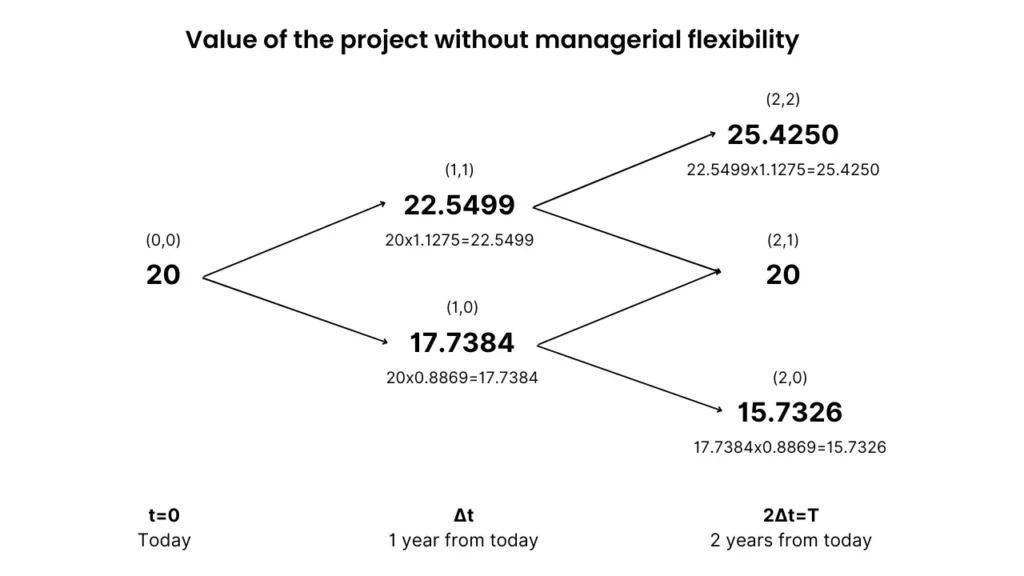
This means that at year 1 for example, the project will either be valued at $22.5499 million with a 59.66% chance (risk-neutral probability) or drop down in value to around $17.74M.
We went from left to right to see how the project’s value (underlying asset price) can change over time.
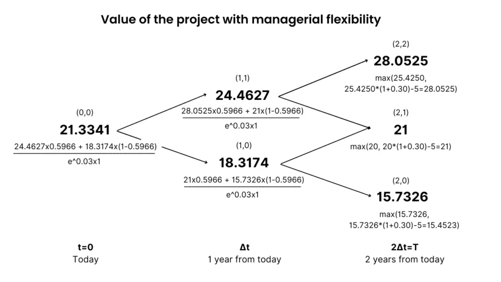
Now, to get the value of the project with the real option we go from right to left.
We start by introducing the option to expand (30% gain and $5M additional investment cost) on the three nodes at the expiration date.
Then, we can get the value—node (0,0)—through a series of backward calculations using the risk-neutral probability of an up move in the following formula:
Where fi,j is the node you’re calculating, qu is the risk-neutral probability of an up move, and e-rΔt discounts the value for one period assuming continuous compounding.
What we’re doing is taking the expected value between nodes and discounting it for one period using the risk-free rate.
Once you get to node (0,0) you have the total value of the investment project with managerial flexibility.
Here’s what that looks like on our binomial tree:
What are those max()?
Remember, the intrinsic value of a financial call option at expiration is the maximum between these two values:
- Zero, as the right (but not the obligation) to something can’t have a negative value.
- The difference between the underlying asset’s price and the strike price.
Let’s translate this to real options:
The value of the project including the option to expand will always be at least equal to the value of the project without it.
In this case, the project value at expiration is the greatest value between having no managerial flexibility, and that value plus the 30% gain minus the $5M cost.
For example, for the (2,2) node, the value of the project without flexibility is around $25M. With flexibility it shoots up to $28M. This means in that scenario, exercising the option is a good investment decision.
For the (2,0) node however, the project’s worth including the option is lower than without it, thus the company won’t expand.
Similarly, you can also calculate the value of the option to expand (option premium) separately:
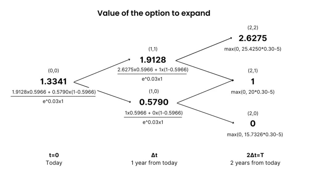
Both ways will give you the same expanded NPV:
Expanded NPV = Project value with flexibility – Initial investment = 21.33 – 16 = $5.33M
Expanded NPV = Static NPV + Option value = 4 + 1.33 = $5.33M
Ultimately, the goal is to help the manager decide if she should take the option to expand or not. The real options decision tree tells you when to exercise the option to expand:
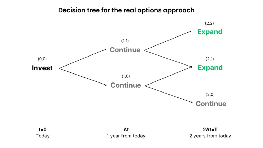
As you can see, there’s one scenario where the manager won’t exercise the option to expand.
Using the Black-Scholes Model
Because this is an European option (can only be exercised at expiration), you can also use the Black-Scholes model to price the real option.
The Black-Scholes model is basically the binomial model if you take the number of steps to infinity.
It relies on the cumulative normal distribution function to make its computations:
Where:
- S0 is the spot price of the option. In this case it is the increase in value from the option to expand, so 20×30%=$6M.
- K is the strike price (expansion cost).
- r is the risk-free rate.
- σ the volatility of the project’s value.
- T the time to expiration, which is 2 years.
Next, you take the values of the d1 and d2 parameters to a cumulative normal distribution table to find the probability of the underlying asset price being above the strike price of the option at the expiration date.
N(d1) is 0.9348 and N(d2) is 0.9104. You use these values to calculate the value of the call option:
Thus, the expanded NPV is:
Expanded NPV = 4 + 1.3222 = $5.32M
Which is really close to the results we got from the binomial model.
#2) Option to Abandon Example
For the second real options analysis example, we’ll be valuing the managerial flexibility of an option to abandon.
Imagine:
- A company that will run a project for two years and then sells it at its fair price.
- The project has an initial investment of $200 million.
- The present value of expected cash flows without flexibility is $195 million, with an annual volatility of 20%.
- The company can sell the remaining assets of the project at any time during the two years for $180 million.
- The risk-free rate is 5%.
The option allows the company to abandon operations at any time. By definition, it only exists once you are in the project and pay the initial cost.
“At any time during the two years” means this is an American put option. As such, we can’t use the Black-Scholes model.
We’ll use a two-step binomial model again. The up factor (u), down factor (d), and risk-neutral probability of an up move (q) are the following:
And the resulting binomial tree without the value of managerial flexibility is:
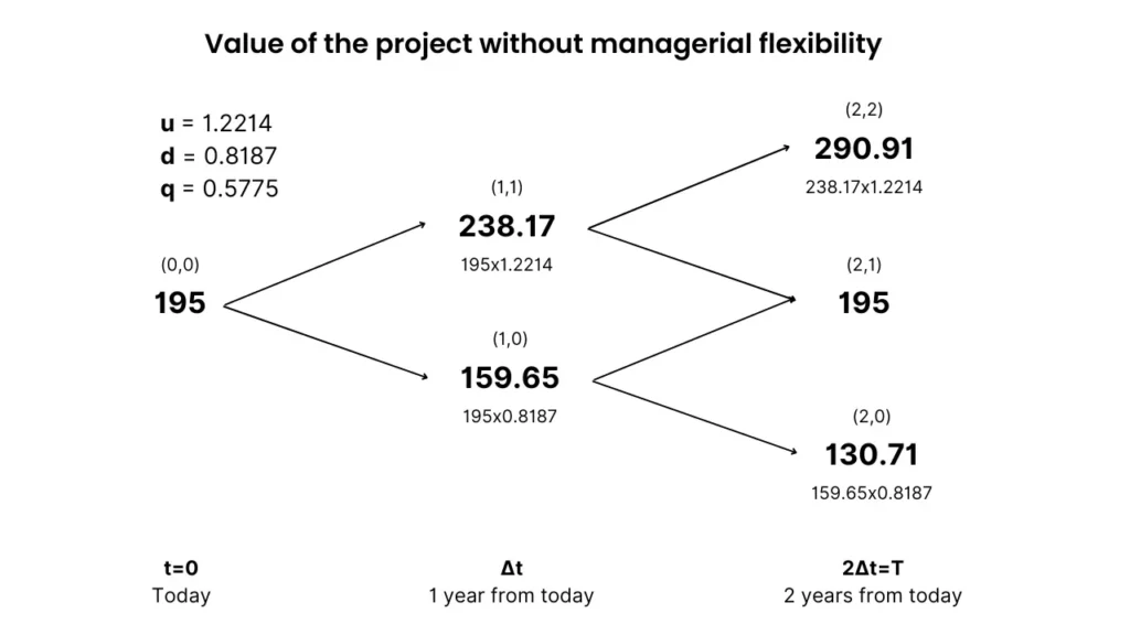
With a present value of expected cash flows of $195M and an investment cost of $200M, the static NPV is negative -$5M, which signals the business shouldn’t move forward with the project because it destroys value.
But will the expanded NPV be positive? Let’s include the option to abandon for the salvage value of $180M in the total project value and see what happens:
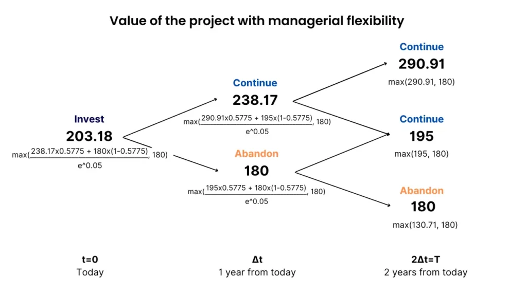
The expanded NPV is 203.18 – 200 = $3.18M, which is positive and thus indicates the company should invest, provided it has an abandonment option.
Let’s break down some things you might be wondering:
Because this is an American option, the value of the project at each node will be the bigger value between having flexibility and not having it (in this case, the PV of cash flows vs. the salvage value). As opposed to only considering this at the maturity date (European options).
One year from today, the manager will ask himself: “Should we wait one more year to see how things pan out, or should we shut down the project right here?”
If the company abandons the project in the first year, it recovers $180M and loses the chance to see the investment rise to $195M. That is, once the manager decides to abandon the project, it obviously ceases to exist. He can’t abandon the same project twice.
As an example, if things go well and the node (2,2) scenario materializes, $290.91M is the present value of the cash flows at that point in time. The company gets that value, instead of the $180M recovery value.
But if things go bad in the first year and the manager lets the project run until the 2nd year (2,0)? The company can still exercise its real option to abandon (put option).
It has the right to sell the project for $180M. If it didn’t have this option, it would have to sell it for $130.71M, losing around 70 million dollars as opposed to $20 million.
The put option does a tremendous job of cutting losses.
Do you see the power of the real options framework?
The option to abandon a project at any time and recover $180M is immensely valuable.
Most projects in the real world are like this. You can abandon them at some point and recover some value. Managers should take that value into account in their decisions.
#3) Option to Contract Example
The last example of real options in capital budgeting deals with an option to contract.
- Initial investment: $150,000
- Present value of cash flows without flexibility (underlying asset): $140,000
- Volatility of the underlying asset: 15%
- Time to maturity: 2 years
- Decrease in project value by exercising the option to contract: 35%
- Residual value (strike price): $50,000
- Risk-free rate: 4%
The firm is considering the option to contract only in two years’ time. Thus, this is an European-style option.
An option to contract reduces operations, thus recovering the scrap value of the assets no longer needed.
It works as a put option, but only for a fraction of the value of the project.
Using Excel and the Black-Scholes model:
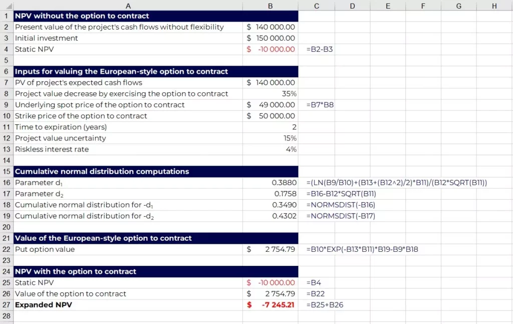
In this example, the company should not go ahead with the project as both the static and expanded NPV are negative, meaning the investment destroys value for the firm.
Real Options FAQs
What is the real options approach?
The real options theory in strategic management and project valuation refers to the opportunity to change operating strategy to take advantage of future good news and cut the effects of bad news. Although this flexibility is very valuable, it is not considered in standard discounted cash flow (DCF) models.
What are examples of real options in business?
The major types of real options in capital budgeting include the option to expand a project that is going well, the option to abandon a project that is going bad (and recover some real asset value), and the option to contract an investment also going bad. Other real options types are the option to delay, restart, or shutdown a project.
Is a stock option a real option?
No. Real options refer to the value of the flexibility to change the course of a real-world project, generally involving physical assets. Thus, the underlying asset is the expected value of the project. A stock option on the other hand, is a financial option, for which the underlying asset is an intangible asset.
