Utility theory in finance measures how much benefit you, as an investor, get from a given asset, and how that will affect your decision to buy that asset over another.
We know supply and demand determine the price of an asset.
Utility theory looks at demand. It studies what makes an investor buy a risky asset, and how he chooses between different assets.
In this post, we’ll start by understanding the preference humans have for smooth consumption, which is important to know how to interpret the graph of a utility function. Then, we’ll see how to evaluate cash flows that are certain (as opposed to uncertain).
Unfortunately (or fortunately), the real world is uncertain. A better approach is needed and that’s where expected utility theory comes in.
Let’s dive in:
Smooth Consumption
Let me ask you this:
Let’s say you have two options over how you will organize the way you eat over the next 4 weeks. You can either choose:
- Moderation: Eat 3 meals (breakfast, lunch, and dinner) a day every day for the next 4 weeks.
- Feasting: For 2 weeks, you eat 6 meals a day (2 breakfasts, 2 lunches, 2 dinners). After every single meal your stomach is so full you that look like you’re minutes away from birthing 2 beautiful twins. For the remaining two weeks you don’t eat a thing. You starve.
Which one would you choose?
Even though the total amount of food consumed over the 4 weeks is the same, you will choose option 1. Why?
The value you get from eating moderately every day is superior to the value you get from feasting for two weeks and starving for the next two. Again, the monetary value of the food is the same. The benefits you get from these two consumption paths is not.
This is the concept of smooth consumption:
People prefer a stable path of consumption. We want to save some of our consumption from periods of abundance to periods of scarcity to get more stability and predictability.
There are many states of the world, which means many potential outcomes can occur throughout your life. To reduce this uncertainty, you choose to give up some consumption today to prevent a negative outcome in the future.
The utility function represents the benefit a consumer gets from a particular bundle of goods and services.
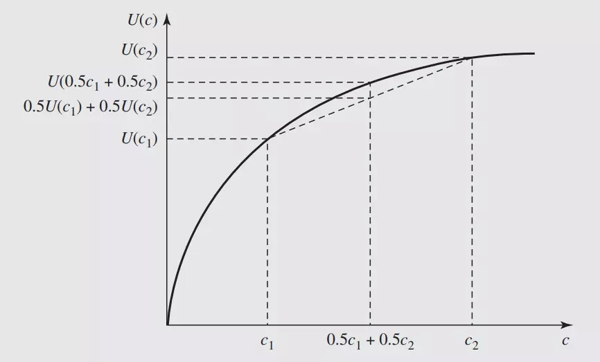
Continuing the example from above, c1 is the consumption in the first two weeks and c2 in the last two. U(c1) and U(c2) represent the utility (benefit) you get from a given consumption period (c1, c2).
Preference for consumption smoothness means we prefer consuming (c1, c2) = (4, 4) over the alternative (c1, c2) = (3, 5). This means U(4) + U(4) > U(3) + U(5).
The sum is the same, but the benefit you get as a consumer is not.
State Dominance
A risky investment is one that generates a stream of uncertain future cash flows.
You will receive more or less depending on what happens from the moment you make the investment to the future.
Let’s step into a theoretical world for a second where:
- There are only two future states of nature.
- The probability of either state happening is the same (50%).
- You know the future value of the investment given the different states.
Something like this:
| Cost Today ($) | Value Tomorrow ($) | ||
|---|---|---|---|
| θ = 1 | θ = 2 | ||
| Investment 1 | –1,000 | 1,100 | 1,200 |
| Investment 2 | –1,000 | 700 | 1,400 |
| Investment 3 | –1,000 | 1,100 | 1,400 |
θ is the Greek letter theta. It represents the different states of nature. Each state of nature has a certain probability (π) of happening. In this case we say it’s 50%.
Which one of these three investments is the best?
Investment 3 clearly dominates both other investments. It pays more or at least the same in both states of nature.
We call this state-by-state dominance, and it is the strongest possible form of dominance.
We assume the typical individual desires a bigger payoff, as it allows them to get more, rather than less, consumption goods.
Now, if you compare investments 1 and 2, you’ll see neither one dominates the other. Investment 1 performs better in state θ = 1, and investment 2 performs better in θ = 2.
Investment 2 is riskier, as its payoffs vary more. However, this does not mean everyone prefers 1. Risk is not the only consideration.
The ranking between the two projects depends on the preferences of each individual. This is why dominance is an incomplete way of ranking prospects.
On top of that, we rarely know what the future states of nature are, let alone their probabilities, let alone the returns in each state.
We need a more general way to compare random potential returns:
Utility Theory in Finance
We start by defining what is a utility function in finance:
Existence of a Utility Function
Investors are able to compare different bundles of goods and services.
For two bundles a and b, there’s a preference relation:
This expression means the investor in question prefers bundle a over bundle b, or is indifferent between them. Pure indifference is represented by a ⁓ b, and strict preference by a > b.
This preference guarantees the existence of a utility function:
This means a utility function is a representation of an investor’s preferences among different bundles.
The notion of a bundle is very general. Different elements of a bundle can represent the consumption of the same good or service in different time periods. For example, do you prefer ice cream in the summer or in the winter?
A bundle can also be something uncertain.
The problem is under uncertainty, ranking bundles of goods involves more than pure individual preferences. Why? Because the probability of a thing happening affects our preference for that thing.
We need to separate pure preferences from probability estimatations:
Choice Theory under Uncertainty
When we talk about uncertainty, our focus is on payoffs dependent on different future states of nature, as opposed to bundles with known characteristics.
We assume individuals have no preference for the assets themselves (not 100% true in reality), but rather they are interested in the payoffs these assets will yield and with what likelihood. The higher the payoff, the better.
Of course, investors don’t know today which asset will yield the higher payoff tomorrow (when the state of nature is revealed).
They have to choose probability distributions that represent these payoffs. A frequently used proxy for a future return distribution is its historical distribution.
As an investor, you can imagine different possible scenarios. Some of which will result in a higher return for one asset, while other scenarios will favor other assets.
Going back to the example above, we said the probability of both is 50%. What happens if we change this? The more likely is state 1, the more attractive Investment 1 is.
Typically, no one investment prospect will strictly dominate the others when they’re uncertain.
How do we choose then?
There are two ingredients in the choice between two alternatives:
- The probability of the future states of nature.
- The level of utility you get from the investment after it’s completed.
Knowing this, we can compute a utility function ![]() :
:
pA is a random value given by a distribution. It changes according to the state of nature θ1 or θ2. π is the probability of a state of nature happening.
In this case, there are only two states, but there can be more. Many more. To the point we can use a summation with the Greek letter sigma.
The utility function of the asset is the expected value of the random values. The expected value of a random value is a value given by its probability distribution multiplied by the probability of the state of nature associated with it.
The utility of an asset with uncertain payoffs is proportional to the probability of the state of the uncertain payoff happening.
In other words, we are computing the weighted average of the utilities of the uncertain payoffs, using the probability of the states of nature as weighs.
![]() (pA) is a real number. However, it doesn’t mean anything. It only has meaning when compared to other assets you’re considering, as it’ll allow you to rank them in terms of their utility.
(pA) is a real number. However, it doesn’t mean anything. It only has meaning when compared to other assets you’re considering, as it’ll allow you to rank them in terms of their utility.
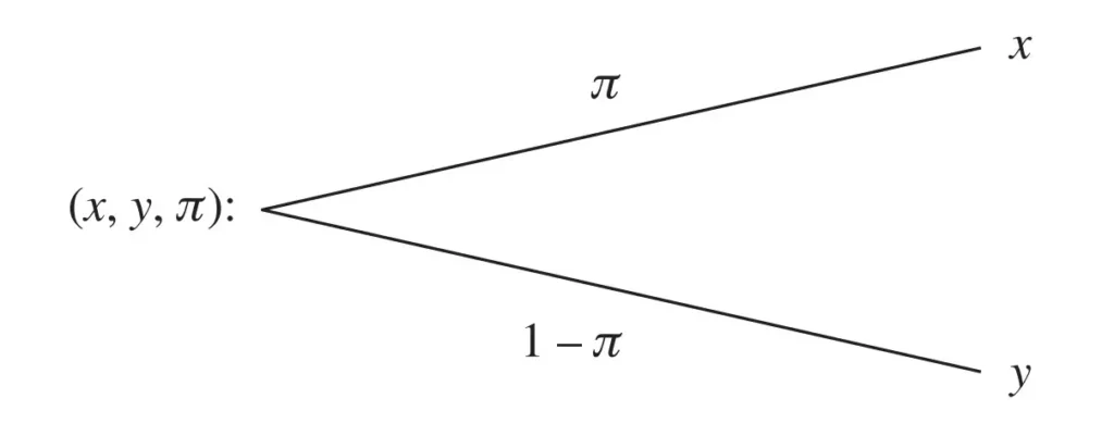
We can represent this more simply with a lottery:
Expected Utility Theorem: Understanding Lotteries
A generic lottery is expressed by (x,y,π).
It offers payoff (consequence) x with probability π and payoff (consequence) y with probability 1 – π.
This notion of a lottery is general and encompasses a variety of possible payoff structures, including other lotteries. This will create a compound lottery—similar to how a binomial tree works.
Lotteries also include individual payments. For example, (x,y,π) = x if (and only if) π = 1.
Knowing this, there’s a utility function ![]() , with the corresponding utility-of-money function U(), such that:
, with the corresponding utility-of-money function U(), such that:
The overall ![]() is defined over lotteries and is the von Neumann—Morgenstern (VNM) utility function. U() is the utility-of-money function (or simply utility function).
is defined over lotteries and is the von Neumann—Morgenstern (VNM) utility function. U() is the utility-of-money function (or simply utility function).
These two are not the same.
We define the VNM utility function over uncertain asset payoff structures, while its associated utility function is defined over individual money payments.
The Bottom Line
Consumption-smoothing plays a major role in the demand for securities.
You get a bigger benefit from smooth consumption, even though the amount you’re consuming is the same. You’re just spreading it over time, instead of spending it all now and suffering later.
Risk means uncertainty in the future cash flow stream. The cash flow of an asset in any future period is typically modeled as a random variable.
The expected utility theory is the pillar of choice theory under uncertainty. Expected utility is a straightforward, intuitive method for comparing uncertain asset payoffs. This allows us to rank the assets themselves.
Two ingredients are necessary for this process:
- An estimate of the probability distribution dictating the asset’s uncertain payments.
- An estimate of the investor’s utility-of-money function. This is what fully characterizes his preferences when ranking different assets. In other words, how risk averse is the investor?
The number given by a utility function doesn’t mean anything standing by itself. Only when compared.
