Optimal Risky Portfolio: 5 Things You Must Understand

The optimal risky portfolio (also called tangency portfolio) is a portfolio composed of risky assets in which the amount you invest in each asset will make it so the portfolio gives you the highest possible return for a given level of risk.

Want to better understand this? Learn these 5 things:

#1) Efficient Frontier

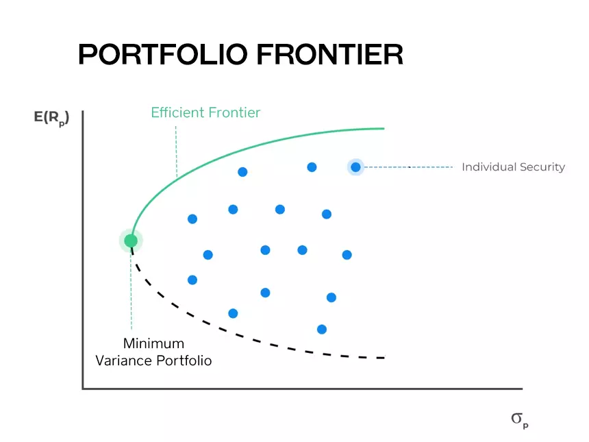
A portfolio frontier (or minimum variance frontier) is a graph that maps out all possible portfolios with different asset weight combinations with minimum risk (variance, or standard deviation) for all given levels of expected return.

The risk of the portfolio is graphed on the x-axis, and the expected return of the portfolio is on the y-axis.

As an investor, you like a higher return, but dislike a higher risk.

This is where the concept of an efficient frontier comes in. The efficient frontier contains the portfolios that dominate all others on the portfolio frontier. It is the upper half of the hyperbola in the graph above. The upward-sloping portion of the portfolio frontier.

What does this mean? It means they give you higher returns for the same level of risk. In other words, the mean of the returns of these portfolios is higher, while the variance is lower.

No rational mean-variance investor chooses to hold a portfolio not located on the efficient frontier.

The portfolios on the efficient frontier provide the highest possible return for a given level of risk.

Now, there are many portfolios in the efficient frontier. Choosing one of them depends on the investor’s risk aversion and utility function.

A portfolio above the efficient frontier doesn’t exist, while a portfolio below the efficient frontier is inefficient.

The minimum risk portfolio—also called MVP (Minimum Variance Portfolio), because it is the variance of an asset’s returns that determines the risk of the asset—is the portfolio with the least risk. This implies it has a lower expected return too though.

The MVP is located on the point that is most to the left on the portfolio frontier.

#2) Optimal Risky Portfolio with Two Risky Assets

The frontier for a portfolio of two risky assets will vary according to the correlation between the two.

If the assets have perfect positive correlation (ρ = 1), the efficient frontier is linear. The two assets are identical, and there are no gains from diversification. This is unrealistic. In the real world, two assets with perfect correlation are actually the same asset.

If the assets have perfect negative correlation (ρ = –1), the minimum variance portfolio is risk-free because the asset’s risks cancel out each other. This also doesn’t happen in reality.

When the assets have imperfect correlation (between –1 and 1, but not equal), the risk of the portfolio is lower than if the assets have a perfect positive correlation.

Why?

Because there are gains from diversification. This is the most realistic case. It’s unlikely you’ll find perfect correlation in the real world between two distinct assets.

In order to understand how diversification reduces the risk of a portfolio, let’s take a look at some formulas.

The expected return of a portfolio—E(R_P)—is the weighted average of the expected returns of the assets composing the portfolio:

E(R_P) = w₁E(R₁) + w₂E(R₂)

The same is not true for the variance, which reflects how risky a portfolio is. The formula is different. The variance of a portfolio is generally smaller than the weighted average of the variances of individual asset returns of the portfolio.

This means you can gain from diversification because you can reduce the risk of your portfolio without necessarily giving up higher returns.

The formula for the variance of a portfolio (σ²_P) of two assets is the following:

σ²_P = w²₁σ²₁ + w²₂σ²₂ + 2ρ(R₁,R₂)w₁w₂σ₁σ₂

Notice how the only number that can be negative (and thus reduce the variance of the portfolio) is the correlation (ρ). Low or even negative correlation means more diversification, which means less risk.

To further understand this, let’s look at the efficient frontier for two imperfectly correlated risky assets:

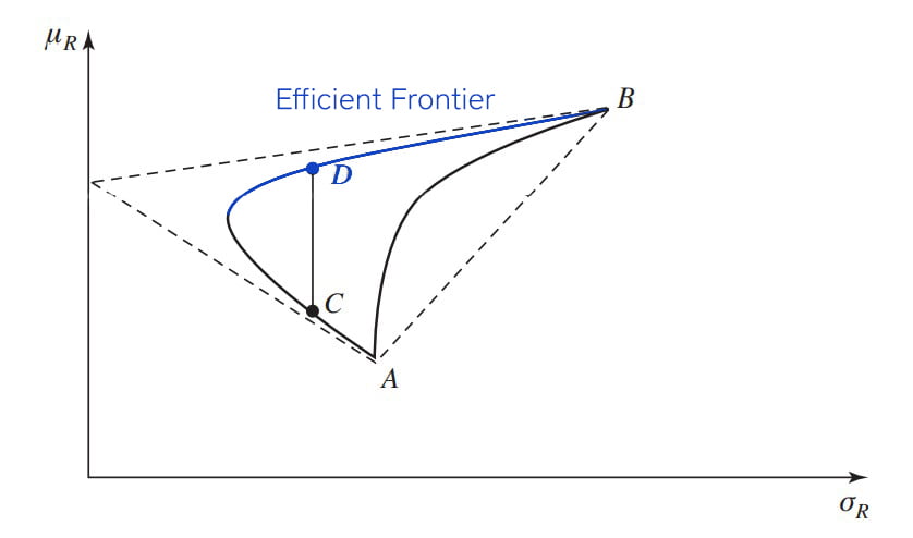
All portfolios between A and B belong to the minimum variance frontier.

Portfolio D dominates portfolio C because it provides a higher return for the same level of risk, hence it is more efficient. This doesn’t happen when the assets have perfect positive correlation, as all portfolios are efficient in that case.

Portfolio B is the riskiest, but also the one with the highest expected return.

The smaller the correlation (the further away from positive 1), the more to the left the efficient frontier is. For example, the assets in portfolio D have a lower correlation (probably negative) than the assets in portfolio B. In other words, less correlation between assets results in lower risk because of diversification.

The dashed lines convey the perfect correlation cases seen before.

Now, let’s understand how a risk-free asset affects the portfolio:

#3) Optimal Portfolio with a Risk-Free Asset

When you introduce a risk-free asset to a two-asset portfolio, things change. You now have a complete portfolio.

A risk-free asset is one that has a certain future return. In reality, you can argue these don’t exist, but in general we consider government bonds from developed countries risk-free assets.

If one of the two assets is risk-free, the efficient frontier is a straight line, as opposed to being the upper half of a hyperbola. This line originates from the return of the risk-free asset in the y-axis.

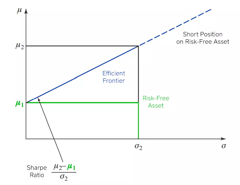
The Sharpe ratio is the slope of the line and it measures the increase in expected return per additional unit of risk (standard deviation).

Now:

Remember that a portfolio is also an asset in it itself. It is defined by its expected return, its standard deviation, and its correlation with other assets or portfolios.

Thus, the previous analysis with just two assets is more general than it seems:

You can easily repeat it with one of the two assets being a portfolio. This means you can extend the analysis from two to three assets, from three to four, and so on.

If there are n (infinite) risky, imperfectly correlated assets, then the efficient frontier will have a bullet shape:

With more and more assets, diversification possibilities improve and, in principle, the efficient frontier is more to the left.

Your goal is to maximize the expected return per unit of risk. Or in other words, the Sharpe ratio.

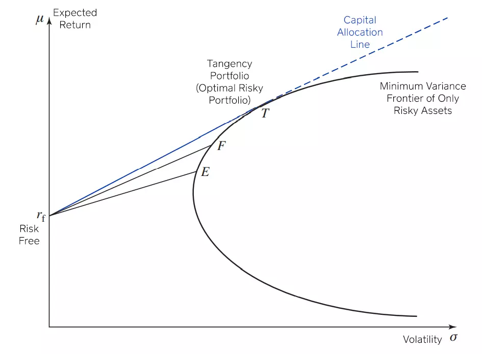
You want to find the capital allocation line with the highest possible slope, but for a portfolio that still exists. This means you want to find the line that is tangent to the bullet shape.

For example, portfolio E is composed solely of a bunch of risky assets. If we combine this portfolio with one risk-free asset, we get the straight line originating from the risk-free return to point E.

You can quickly check that all portfolios on this line are dominated by those you can create by combining the risk-free asset with portfolio F. All portfolios on the line ending in F have a higher expected return for the same risk level (volatility) than the portfolios on the line ending on E.

Keep searching for the highest similar line combining the risk-free return with the risky asset bullet-shaped frontier and you obtain the truly efficient frontier—the straight line originating from the risk-free return on the y-axis that is tangent to the risky asset frontier.

This is the Capital Allocation Line:

Capital Allocation Line

The capital allocation line (CAL), also called global efficient frontier, is a line that reflects the best combinations of risky assets with a risk-free one. This line only exists when the portfolio contains a risk-free asset, like a government bond for example.

It is a straight line tangent to the bullet-shaped frontier of risky assets. The y-intercept of the capital allocation line is the risk-free rate.

Every single point on this line is a portfolio of risky assets that includes a position on the risk-free asset, except for the tangency portfolio (also called the optimal risky portfolio).

The T in the graph above is the tangency portfolio. This portfolio is the only portfolio on the capital allocation line composed solely of risky assets, hence why it is also called an optimal risky portfolio. As before, if short positions in the risk-free asset are possible, the efficient frontier extends beyond T (dashed line).

A short position in the risk-free asset is, for example, a loan where you pay the risk-free interest rate. This means the portfolio can be riskier than the riskiest of assets that compose it because of leverage. This is why it goes off to the left without end. More risk, more return.

To the right of the optimal risky portfolio, the position on the risk-free asset is a deposit.

#4) Optimal vs. Efficient Portfolio

Optimal risky portfolio can have a different meaning though:

When we say a portfolio is optimal, we are talking about a portfolio that maximizes the preferences (utility theory) of a given investor.

This is different than saying a portfolio is efficient. An efficient portfolio is any portfolio on the efficient frontier. The optimal portfolio is one of the portfolios that make up this frontier, based on the preferences of the investor.

Imagine two investors who share the same perceptions as to expected returns, risk, and return correlations for a pair of assets but disagree in their willingness to take risks.

The efficient frontier will be identical for these two investors. However, different points on that same line (frontier) will represent their own personal optimal portfolios.

Because they have different preferences the optimal risky portfolio for each is different.

It’s also important to talk about the difference between optimal risky portfolio and optimal complete portfolio.

An optimal complete portfolio is any portfolio in the capital allocation line that includes risky assets and risk-free assets. On the other hand, the optimal risky portfolio is also on the capital allocation line, but it is only composed of risky assets. This is the only point on the CAL with this characteristic.

#5) How to Calculate the Optimal Risky Portfolio

To calculate the optimal risky portfolio for more than two assets, you need to understand matrixes and vectors. On top of that, the returns of these assets must be linearly independent—you can’t write one as a linear combination of the other.

Otherwise, this results in a matrix for which you can write one of the rows as a combination of the others (singular matrix). The problem is you cannot invert singular matrixes, which is something you’ll need to do below.

The optimal risk portfolio formula is a vector of weights of the assets that compose it, and is given by:

\[w_T^*=\frac{1}{A-Cr_f}V^{-1}(\overline{r}-r_f1)\]

Where:

\[A=1^{T}V^{-1}\overline{r}\]

\[B=\overline{r}^{T}V^{-1}\overline{r}>0\]

\[C=1^{T}V^{-1}1>0\]

\[D=BC-A^{2}>0\]

On top of that, 1 is a vector of ones. How many ones? The same as the number of assets. V is the covariance matrix of returns. is the vector of expected returns for each asset. rf is the risk-free rate.

The optimal portfolio weights must add up to 1, as the weight of the risk-free asset is zero. For the other portfolios on the CAL that are not the tangency portfolio, the weights will add up to less or more than one.

Here’s why:

When the portfolio is located to the left of the optimal risky portfolio, the weights for the risky assets add up to less than 1, indicating a positive weight for the risk-free asset (deposit). For portfolios to the right, they’ll add up to more than 1. The difference indicates the negative weight for the risk-free asset (borrowing). When you add this negative weight to the others, it will give you 1.

The vector of expected returns for the tangency portfolio is:

\[\mu_{T}=r_f+\frac{H}{A-Cr_f}\]

Where:

\[H=(\overline{r}-r_f1)^{T}V^{-1}(\overline{r}-r_f1)\]

How to Find an Optimal Risky Portfolio in Excel

To find the optimal risky portfolio in Excel, you want to maximize the Sharpe ratio. To do that you can use the Solver add-in.

To find the tangency portfolio you need:

• The expected return and risk of all assets that compose the portfolio.
• The covariance matrix between them.

Using Solver, maximize the Sharpe ratio by changing the weights invested in each asset.

Frequently Asked Questions (FAQs)