Potential Future Exposure: Definition, Calculation, Example

Potential Future Exposure estimates the most you can win in a trade within a given timeframe and with a given confidence level. By extension, it tells you the most your counterparty can end up owing you, exposing you to the risk they fail to pay. PFE is mostly used by banks selling derivatives to other firms.

That’s the gist of it.

Still confused? Keep reading:

What Is Potential Future Exposure

Potential Future Exposure (PFE) is the maximum expected market risk exposure to a portfolio of derivative transactions at a chosen confidence level.

What is exposure exactly though?

A firm has credit exposure to its counterparty in a trade when the firm wins the trade.

Imagine two banks trading a derivative. Bank A is buying an option from Bank B.

If Bank A loses the trade (the option it bought expires out of the money), Bank B defaulting in the meantime is irrelevant. Because Bank B doesn’t owe Bank A any money.

Credit exposure would only exist if Bank A won the trade (the option expired in the money). Why? Because if Bank B defaults before the contract’s expiration, Bank A will have trouble receiving its winning cash flow from the trade.

In essence, only a gain exposes a firm to counterparty default.

At the beginning of the contract, neither bank has exposure to the other as there’s no initial cash flow (unless a premium or margin is charged). Derivatives have no value at the time of their creation.

In contrast, the real exposure a bank faces when giving out a loan exists since day zero of the contract, and it is straightforward to calculate—it is the full capital amount lent out to the counterparty at the start.

Additionally, exposure is unilateral as only the lender is exposed to the borrower, unlike in a derivatives contract where exposure is bilateral (can swing negative or positive for either party).

Also, the credit exposure in a bank loan starts at a known fixed amount and decreases as the counterparty makes its capital payments, while in a derivatives trade, exposure varies up and down throughout the life of the contract according to market fluctuations (in the underlying asset) that are impossible to predict with 100% certainty.

The goal of PFE is to estimate these potential future fluctuations.

And then derive the maximum loss that can occur when a trade goes in your favor, and your counterparty ends up owing you money.

Banks selling over-the-counter derivatives to other firms often use PFE to understand the counterparty credit risk they face.

The goal is to set a maximum PFE limit for a portfolio of derivative transactions to cap the risk for the bank in case the counterparty defaults and is unable to pay its obligations.

This limit is the maximum estimated exposure the bank is okay with, depending on the size and risk profile of the counterparty and the instruments traded.

Let’s understand how to calculate potential future exposure:

How to Calculate PFE

There are different ways to estimate future exposure, the most common way being through the VaR (Value-at-Risk) methodology using a Monte Carlo simulation.

The Monte Carlo simulation creates a probability distribution of likely returns. It simulates the price path of market parameters that influence the value of the derivative.

To accurately model exposure and how it evolves over time, it is key to choose the correct parameters that influence the value of the trade.

For instance, in an interest rate swap the main parameter considered is the variable interest rate. In a foreign exchange derivative it will be the underlying exchange rate. And in an options contract the underlying asset (along with the Greeks).

It’s impossible to know with certainty how these risk factors will behave at a future date.

What a Monte Carlo simulation does is simulate thousands of potential price paths for these risk factors. How so?

Through a stochastic model like the Geometric Brownian motion (GBM).

A stochastic model forecasts the probability of an outcome under different conditions, using random variables (risk factors). It simulates thousands of possible future market scenarios.

The second step after running the model is to price the value of the derivatives contract in each scenario.

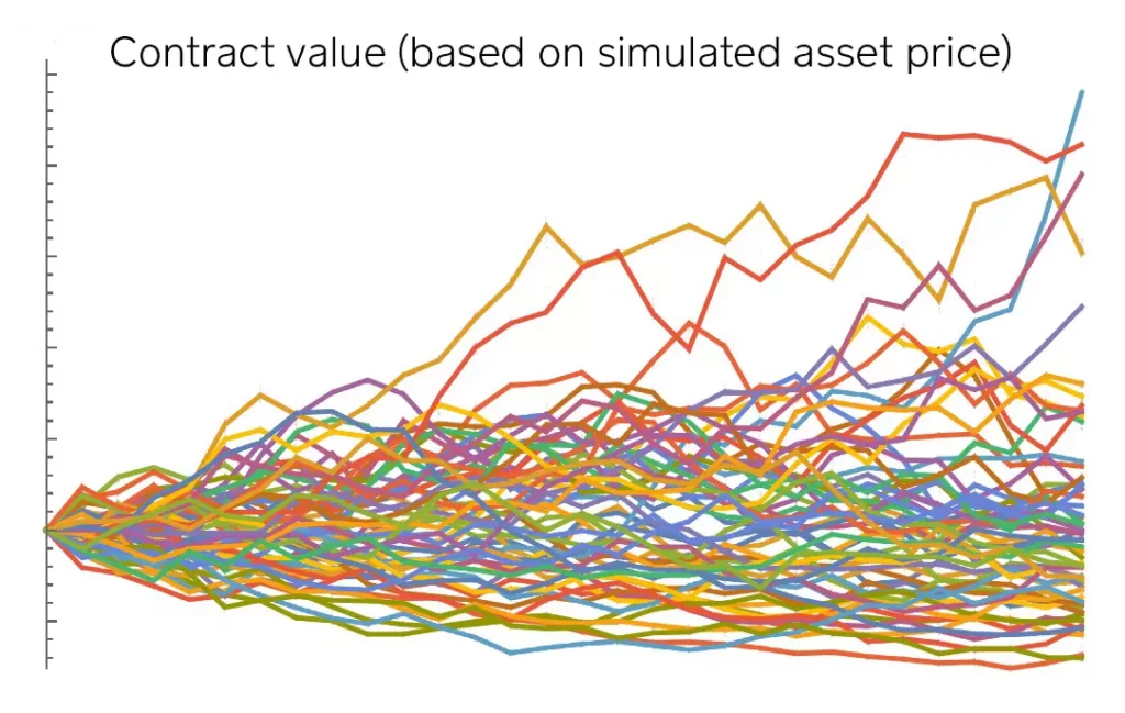
Each scenario (determined by the chosen risk parameters) implies a different value for the contract at each point in time.

In some scenarios, one counterparty is winning while in others it is losing.

For instance, the buyer of an option is losing money in the scenarios where the underlying asset’s price went down, and winning when it went up (all else equal).

But remember, exposure only exists when you are winning the trade. Negative portfolio exposure means no loss even if the counterparty defaults, because you are losing the trade anyway.

Therefore, the scenarios where you are losing money are ignored.

Once you have the distribution of possible future values of the derivatives contract, you focus on the distribution of positive values to get the PFE and delete negative values.

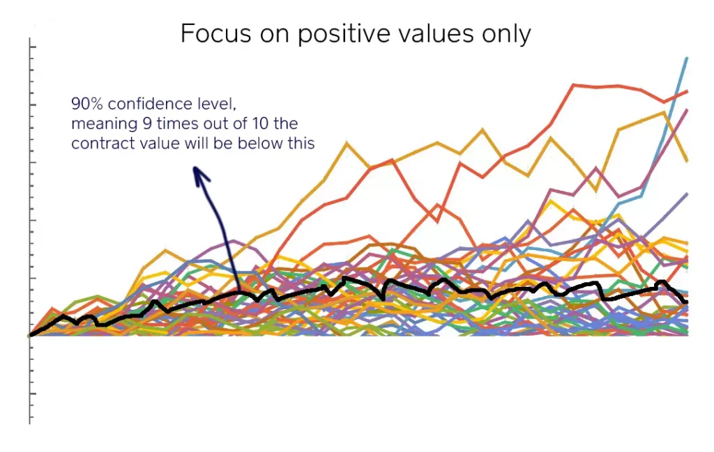
You typically compute PFE as the maximum loss with a 95% (or 99% or 90%) confidence level. This tells you the estimated worst-case replacement cost at every future date.

For instance, for a confidence interval of 99% for instance, the PFE estimate is the largest loss a bank will suffer 99 times out of 100.

In other words, PFE is the most you can lose over the next year with 99% certainty. Similarly, there is a 1% chance you lose more than that value.

That loss value comes from a scenario where the counterparty made a bad bet, the market went the opposite of what they thought, and now they owe you lots of money. You are exposed to the risk of them not affording the payment.

How much would it cost to replace the winning contract at the time of default of the counterparty? That is the exposure.

After deriving that potential replacement cost, banks set a maximum PFE limit to cap their potential losses.

Let’s go through an example to put these concepts in motion:

Potential Future Exposure Example

Imagine a hedge fund with $2B in net assets that wants to trade a 1-month interest rate swap with a bank.

The fund believes the Euribor will decrease within the next month, so it wants to pay the Euribor to the bank and receive a fixed rate.

The firms agree to exchange one interest payment on a given notional amount, one month from today. The bank, the fixed rate payer, pays a fixed rate a month from now. The hedge fund, the floating rate payer, pays the Euribor.

Based on the net assets of the fund, the legal agreements in place, the tenor of the contract, and the riskiness of the fund’s portfolio, the bank sets a maximum PFE limit up until it is ok trading with the fund.

In this case, the bank sets a PFE limit at 5% of the fund’s NAV ($100M).

This means the bank’s traders are allowed to trade with the fund up to that limit. If at any moment while the trade is live, the simulation model returns a PFE (re-calculated every day) above that limit, there’s an excess.

Notice that it is not the notional amount of the trade that counts, nor the value of the contract (who is winning/losing, which is the current exposure). Although these things feed the thing that matters—the PFE simulation.

The notional amount based on which the interest payments are calculated can be $100M or $1B or whatever. As long as the PFE simulation doesn’t surpass the limit, the bank’s traders can continue accepting the fund’s trades.

Now, how does the PFE calculation work?

PFE exists as soon as the swap contract is active.

The bank will run the numbers and simulate thousands of possible price paths for the Euribor rate (underlying asset) in the next month based on a number of relevant market parameters and risk factors related to it.

And then look at how the value of the contract behaves along each of those scenarios (who is winning/losing at each point in time).

After focusing only on the scenarios where the hedge fund loses the trade, the bank looks at the 90th percentile of worst exposure paths (where the fund loses the most).

This 90% confidence level is the same as saying that 9 times out of 10, exposure is expected to stay below that level within the following month.

Once the firms make the trade, there’s potential future exposure every day until the settlement date.

Those daily exposures together make up the exposure path. Maximum PFE is simply the day when the model forecasts the highest exposure (typically closer to the inception date because there’s more time for unfavorable market conditions to materialize).

PFE is re-calculated every day with a decreasing time period.

So if they trade today, it simulates the maximum the trade may go in favor of the bank within one month, then within 30 days, then 29, and so on.

Keep in mind this whole process is automatic, and typically done by banks’ proprietary software that is fed by internal risk models.

Let’s say in this case the maximum PFE is $20M.

This means there’s a 90% chance the fund ends up owing the bank up to $20M. Likewise, there’s a 10% chance of it owing more than that.

And if the fund defaults within the next month, and the $20M-worst-case scenario materializes, the bank will have a hard time getting paid.

$20M is well below the $100M max PFE limit, for now. If the fund wants to increase the size of the trade, the bank’s traders can accept it as long as the max PFE doesn’t surpass the limit.

Also keep in mind that as a client, the hedge fund does not know of the limit the bank has in place.

Key Takeaways (FAQs)