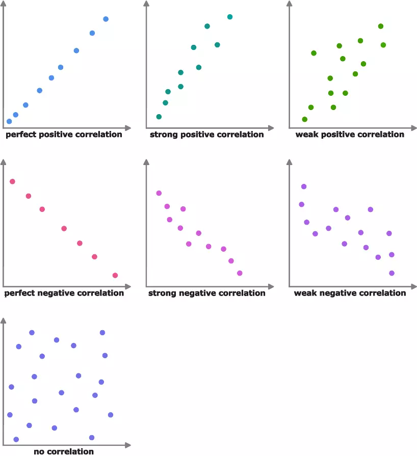
Strict Exogeneity: 4 Essentials About This OLS Assumption

Strict exogeneity is one of the assumptions supporting the Ordinary Least Squares (OLS) method in regression analysis. It states that the explanatory variables are not correlated with the error term of the model. This guarantees the estimated coefficients are unbiased, which is good.

Still confused? Keep reading:

#1) Understanding Strict Exogeneity

In multiple linear regression, the strict exogeneity assumption states that the predictor variables (also called independent, or explanatory variables) are not correlated with the error term.

This assumption is important because it ensures the regression coefficients are unbiased.

The goal of OLS regression is to estimate the relationship between a dependent variable (also called the response variable) and one or more independent variables. How?

By finding the values of the coefficients (parameters) that minimize the sum of the squared differences between the observed and the predicted values of the dependent variable, based on the regression equation. Those differences are the error term.

If the independent variables are correlated with the error term, then the estimated coefficients are biased and the standard errors are incorrect. The problem? Wrong conclusions about the potential outcomes and relationship between the predictor variables and the response variable.

If the independent variables are strictly exogenous, the unconditional mean of the error term is zero. This means that on average, the error term doesn’t have any systematic effect on the dependent variable. You want this to happen because it implies the regression model is correctly specified and the estimated coefficients are unbiased.

The strict exogeneity assumption is part of the Gauss-Markov theorem. Along with other assumptions (such as no perfect multicollinearity), they assure the OLS estimator is the best linear unbiased estimator (BLUE) of the coefficients in a linear regression model.

#2) Example of Strict Exogeneity

Now that we’ve got the strict exogeneity definition out of the way, let’s go through an example:

Let’s say you’re creating a model to see how the temperature on a given day is affected by a number of variables, including sales of a certain product, and concert attendance.

In this case, the temperature is a strictly exogenous variable.

It is not affected by any other variables in the model, such as the revenue of ice cream sales, or how many people go to a certain concert.

However, it’s safe to say that if it’s too hot outside, ice cream sales will go up. And if it rains, fewer people will go to concerts.

The temperature is independent of those variables, but it influences both of them (regardless of the time period).

The causal effect exists only one way. Ice cream revenue and concert attendance don’t affect the temperature in any way. So the temperature is a strictly exogenous variable.

Any dummy variable used in an econometric model is another example of a strictly exogenous variable, in general.

#3) Strict Exogeneity Tests

There are many ways to test for strict exogeneity in estimates. The most common methods include:

The Hausman test, which compares the estimates from a two-step method (such as instrumental variables) with the estimates from a one-step method (such as OLS). If the estimates from the two-step method are not significantly different from the estimates from the one-step method, then the variable is strictly exogenous.

There’s also the Wooldridge test, also known as the Lagrange Multiplier (LM) test. It is useful when dealing with time series data, but also cross-sectional and panel data. The basic idea behind it is that if a variable is strictly exogenous, then the residuals from a regression model are uncorrelated with the lagged values of said variable.

It works by regressing the residuals from a regression model on the lagged values of the variable in question, and then testing whether the coefficients are zero. If they are, then the variable is strictly exogenous. The LM test can’t prove exogeneity, only provide evidence against it.

#4) How to Deal with Endogeneity

Two common ways to deal with endogeneity (independent variable correlated with the error term) include:

• Fixed effects: A fixed effect is a type of regressor used to control for the influence of time-invariant unobserved characteristics on the independent variables.
• GMM estimators: GMM stands for Generalized Method of Moments. It allows you to estimate a parameter even when there’s endogeneity. How? By matching sample moments with population moments.

Strict Exogeneity FAQs